Gaussian Mixtures is a probabilistic latent variable model, that assumes that observed data was generated by sampling from $K$ $d$-dimensional Gaussian distributions.

A problem with K-means is the hard assignments of clusters. It would be nice to have a soft assignment of points to all $K$ clusters, i.e., we would like a probability of each point belonging to each cluster. This is where Gaussian Mixtures come into play.

This algorithm is going to be the first time we see latent variables. In this case, the latent variable could tell what cluster a point belongs to. The algorithm is very similar to Lloyds algorithm in the sence that it also iterates between assigning points to clusters (softly by the use of probabilities) and afterward updating clusters.

Assume, that we have an observation $x \in \mathbb{R}$ and that we would like to know which cluster density produced this observation. To formalize this a bit more, let ${\bf z} = ( z_1, \dots, z_k )$ be a latens variable associated with $x$ and $z_i \in {0, 1}, \quad \sum_{k=1}^K z_k = 1$, i.e., ${\bf z}$ is a vectore of all zeros except for one entry, which is $1$ indicating which of the $K$ clusters that $x$ came from.

Also, let $p(z_k = 1) = \pi_k$ be a prior probability of $x$ coming from each of the $K$ cluster. This implies that $0 \leq \pi_k \leq 1, \quad \sum_k \pi_k = 1$.

We would then like to know what the posterior probability of $x$ is:

This quantity tells us something about the underlying distribution. Now, let’s see if we can somehow estimate this beast.

First, let’s assume, that $p(x | z)$ is a gaussian distribution:

This allows us to rewrite $p(x)$ using the product rule: \(p(x) = p(x | \theta) = \sum_z p(x, z) = \sum_z p(z) p(x | z)\)

Here, $p(z)$ is the (known) prior probability, i.e., $p(z_k = 1) = \pi_k$. Plugging in what we know about $p(x | z)$ and $p(z_k = 1)$ gives us:

This quantity allows us to estimate the distribution over the latent variables. In particular, we can use the product rule again but on the posterior distribution $p(z_k = 1 | x)$.

Note how the last step uses the equality of Eqn. (3). Now we are in a position, where we can try to estimate these quantities. A typical way of doing this would be maximum likelihood. Then we would optimize the following quantity:

Note that we assume here that the $x_i$s are i.i.d. (independent and identically distributed). This problem is not easy. Even the log trick does not work here. So we turn to Expectation Maximization instead, which is a very used and very powerful way of optimizing parameters in latent variable models.

Expectation Maximization

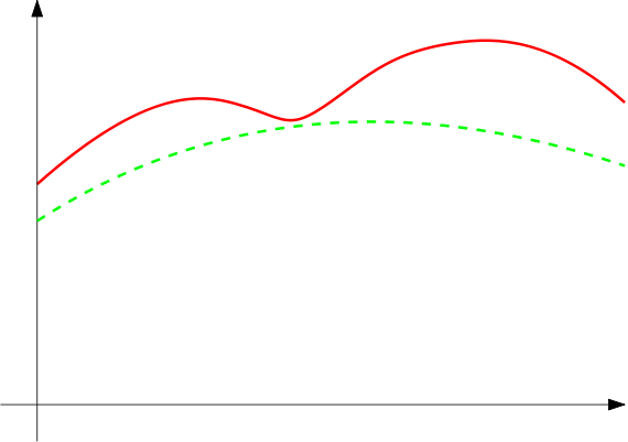
Intuitively, we would like to find a lower bound on the likelihood of the data. This would look something like the following:

Figure 1. Illustration of the lower bound on the likelihood

If we can maximize the lower bound, then we hope to find a good solution for the original problem, which in this case will be the log likelihood $\log p(X | \Theta)$.

To do so, we will have to work with something called free energy. Free energy is defined as follows:

Note how $F$ is a function of both the parameters $\theta$ and a probability density function (pdf) $q$. Now we claim the following:

Hypothesis: Free energy $F(\theta, q)$ is a lower bound for $\log p(x | \theta)$.

If that is actually the case, we can optimize on $F$ instead of the log likelihood in order the estimate the parameters $\theta$.

To prove this hypothesis, we need a very powerful ingredient.

Jensens Inequality: This inequality states that for a concave function $\phi: \mathbb{R} \rightarrow \mathbb{R}$, $\mathbb{E} [\phi(z)] \geq \phi(\mathbb{E} z)$.

Fun fact: Not only is this a very strong theorem. It was also introduced by a dane like my self back in 1906. Probably the most important discovery made by any dane.

Now, we show that $F$ is a lower bound on $\log p(X)$. The proof comes in two steps. First we express $p(X)$ in terms of an expectation and afterward we use the inequality on the log of the expectation.

Taking the log, we can use Jensens Inequality to get the lower bound.

The actual optimization

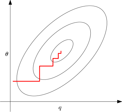
From here, we need to optimize over both over $q$, which is a distribution, and over $\theta$, which is the parameters of our gaussians. So we will need to do an iterative approach to make this work. Visually, it looks similar to the following:

Figure 2. Countour plot of the free energy $F$ that we are trying to minimize. The red curve represents iteratively maximizing over $q$ and $\theta$, holding the other constant. Note how we move along the two axis individually.

To be able to maximize over $\theta$ and $q$, we will first need $F$ in a form where we can actually maximize over the two. In the following, we will rewrite $F$ in two different ways for this purpose.

1. Reformulate $F$ to be able to maximize over $\theta$ for fixed $q$:

Note how the first term is independent of $\theta$ and the second term is essentially $\mathbb{E}_q \log p(x, z | \theta)$. This allows us to maximize over this expectation later.

2. Reformulate $F$ to be able to maximize over $q$ for fixed $\theta$:

This step is a bit more involved. First of all we are going to need another ingredient here. Namely, the KL-divergence:

Kullback-Liebler divergence: This divergence is essentially a meassure of “distances” between two distributions and is defined as follows

As this can be seen as a distance meassure, we can think of the KL-divergence as being minimized, when $p(x) = q(x)$. Now, let’s rewrite $F$:

Again, we don’t care about the first term, when maximizing over $q$ and in order to maximize the negative KL-divergence, we want $q$ to be equal to $p(z | x)$, which we found above in (22), i.e., we let

Putting it all together

Okay, let’s put it all together. We need to do two steps. First, we will select on some initial parameters for $\pi_k$, $\mu_k$, and $\sigma_k^2$. Second, we will iteratively maximize over $q$ (the E-step) and $\theta$ (the M-step).

When initializing the parameters, the most important parameters are the $\mu_k$s that selects the starting point for the $K$ clusters. $\mu_k$s are typically initialized at random. We typically initialize the prior probabilities with $\pi_k = \frac{1}{K}$ and the variances to $\sigma^2 = 1$.

We now cover the E- and the M-step, but first, we will extend the notation a bit. In particular, we let the hidden states $z_i$ be “indicator” vectors $z_1, \dots, z_N \in {0, 1}^K$. By indicator vectors we mean vectors, where the $j$th entry in $z_i$ will be one if $x_i$ was generated from the $j$th cluster. This new notation also gives a slight change in how we write the following already derived quantities. Note, that most of the terms in the products will be 1:

The E-Step

For the E-step, not much need to be done. We already concluded in Eqn. (6), how we would choose $q$. So the only thing that we need to do the actual computations with the current estimates of the parameters.

The M-Step

Above it was stated, that when maximizing over $\theta$, we just need to do it over $\mathbb{E}_q \log p(x, z | \theta)$. Starting from the definition of $p(Z)$ and $p(X | Z)$ we can express $p(X, Z)$ as follows:

We would, however, like to have $\log p(X, Z)$, so lets continue:

Finally, let’s take the expectation over $q$. For this, we use the following equality: In the following derivations, we will use linearity of expectation and this definition: \(\mathbb{E}_q [z_{nk}] = \mathbb{E}_{p(z | x)}[z_{nk}] = p(z_{nk} = 1 | x_n) =: \gamma (z_{nk})\). The equality stems from the fact that $z_{nk}$ is a binary random variable.

The key thing to keep in mind here is that we are currently maximizing over the parameters and so, we have fixed $q$. In turn, $p(z_{nk} = 1 | x_n ) = \gamma(z_{nk})$ is known and can be treated as a constant.

Having found $\mathbb{E}_q \log p(x, z | \theta )$, we can start minimizing the beast. We do this by plugging in the normal distribution and then we can differentiate and set to 0.

First of all, the normal distribution over $x \in \mathbb{R}$ is defined as